Differential Equations with SciPy – odeint or solve |
您所在的位置:网站首页 › scipy solve matrix equation › Differential Equations with SciPy – odeint or solve |
Differential Equations with SciPy – odeint or solve
|
SciPy features two different interfaces to solve differential equations: odeint and solve_ivp. The newer one is solve_ivp and it is recommended but odeint is still widespread, probably because of its simplicity. Here I will go through the difference between both with a focus on moving to the more modern solve_ivp interface. The primary advantage is that solve_ivp offers several methods for solving differential equations whereas odeint is restricted to one. We get started by setting up our system of differential equations and some parameters of the simulation. UPDATE 07.02.2021: Note that I am focusing here on usage of the different interfaces and not on benchmarking accuracy or performance. Faruk Krecinic has contacted me and noted that assessing accuracy would require a system with a known solution as a benchmark. This is beyond the scope of this blog post. He also pointed out to me that the hmax parameter of odeint is important for the extent to which both interfaces give similar results. You can learn more about the parameters of odeint in the docs. import numpy as np from scipy.integrate import odeint, solve_ivp import matplotlib.pyplot as plt from mpl_toolkits.mplot3d import Axes3D def lorenz(t, state, sigma, beta, rho): x, y, z = state dx = sigma * (y - x) dy = x * (rho - z) - y dz = x * y - beta * z return [dx, dy, dz] sigma = 10.0 beta = 8.0 / 3.0 rho = 28.0 p = (sigma, beta, rho) # Parameters of the system y0 = [1.0, 1.0, 1.0] # Initial state of the systemWe will be using the Lorenz system. We can directly move on the solving the system with both odeint and solve_ivp. t_span = (0.0, 40.0) t = np.arange(0.0, 40.0, 0.01) result_odeint = odeint(lorenz, y0, t, p, tfirst=True) result_solve_ivp = solve_ivp(lorenz, t_span, y0, args=p) fig = plt.figure() ax = fig.add_subplot(1, 2, 1, projection='3d') ax.plot(result_odeint[:, 0], result_odeint[:, 1], result_odeint[:, 2]) ax.set_title("odeint") ax = fig.add_subplot(1, 2, 2, projection='3d') ax.plot(result_solve_ivp.y[0, :], result_solve_ivp.y[1, :], result_solve_ivp.y[2, :]) ax.set_title("solve_ivp")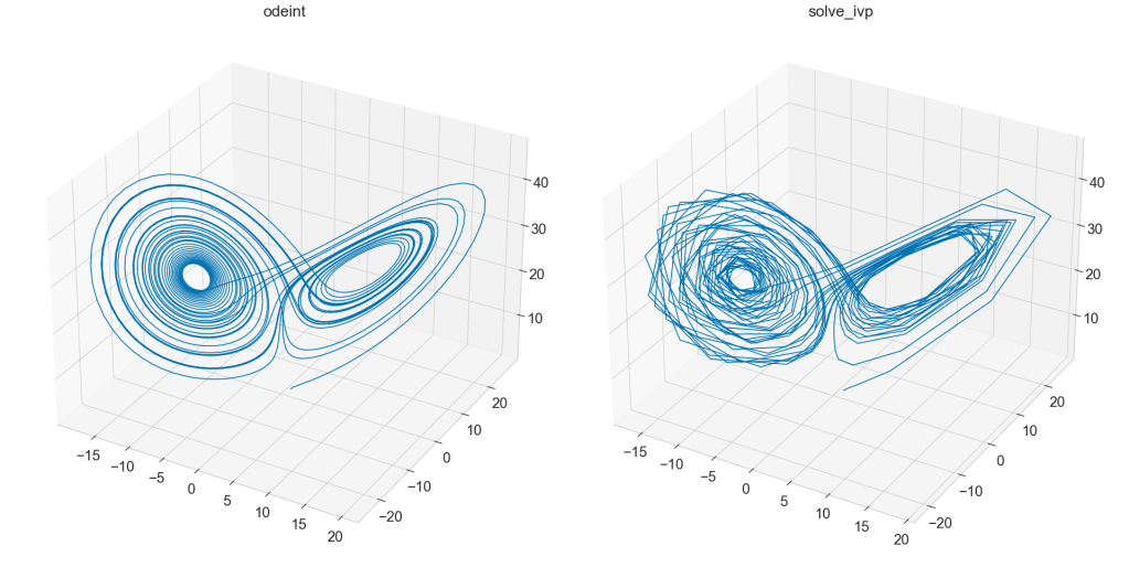 Simulation results from odeint and solve_ivp. Note that the solve_ivp looks very different primarily because of the default temporal resolution that is applied. Changing the the temporal resolution and getting very similar results to odeint is easy and shown below. Simulation results from odeint and solve_ivp. Note that the solve_ivp looks very different primarily because of the default temporal resolution that is applied. Changing the the temporal resolution and getting very similar results to odeint is easy and shown below.
The first thing that sticks out is that the solve_ivp solution is less smooth. That is because it is calculated at fewer time points, which in turn has to do with the difference between t_span and t. The odeint interface expects t, an array of time points for which we want to calculate the solution. The temporal resolution of the system is given by the interval between time points. The solve_ivp interface on the other hand expects t_span, a tuple that gives the start and end of the simulation interval. solve_ivp determines the temporal resolution by itself, depending on the integration method and the desired accuracy of the solution. We can confirm that the temporal resolution of solve_ivp is lower in this example by inspecting the output of both functions. t.shape # (4000,) result_odeint.shape # (4000, 3) result_solve_ivp.t.shape # (467,)The t array has 4000 elements and therefore the result of odeint has 4000 rows, each row being a time point defined by t. The result of solve_ivp is different. It has its own time array as an attribute and it has 1989 elements. This tells us that solve_ivp indeed calculated fewer time points affection temporal resolution. So how can we increase the the number of time points in solve_ivp? There are three ways: 1. We can manually define the time points to integrate, similar to odeint. 2. We can decrease the error of the solution we are willing to tolerate. 3. We can change to a more accurate integration method. We will first change the integration method. The default integration method of solve_ivp is RK45 and we will compare it to the default method of odeint, which is LSODA. solve_ivp_rk45 = solve_ivp(lorenz, t_span, y0, args=p, method='RK45') solve_ivp_lsoda = solve_ivp(lorenz, t_span, y0, args=p, method='LSODA') fig = plt.figure() ax = fig.add_subplot(1, 2, 1, projection='3d') ax.plot(solve_ivp_rk45.y[0, :], solve_ivp_rk45.y[1, :], solve_ivp_rk45.y[2, :]) ax.set_title("RK45") ax = fig.add_subplot(1, 2, 2, projection='3d') ax.plot(solve_ivp_lsoda.y[0, :], solve_ivp_lsoda.y[1, :], solve_ivp_lsoda.y[2, :]) ax.set_title("LSODA")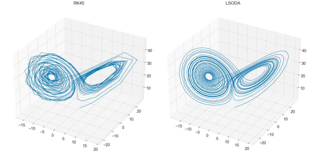 Comparison between RK45 and LSODA integration methods of solve_ivp. Comparison between RK45 and LSODA integration methods of solve_ivp.
The LSODA method is already more accurate but we can make it even more accurate but it is still not as accurate as the solution we got from odeint. That is because we made odeint solve at even higher temporal resolution when we passed it t. To get the exact same result from solve_ivp we got from odeint, we must pass it the exact time points we want to solve with the t_eval parameter. t = np.arange(0.0, 40.0, 0.01) result_odeint = odeint(lorenz, y0, t, p, tfirst=True) result_solve_ivp = solve_ivp(lorenz, t_span, y0, args=p, method='LSODA', t_eval=t) fig = plt.figure() ax = fig.add_subplot(1, 2, 1, projection='3d') ax.plot(result_odeint[:, 0], result_odeint[:, 1], result_odeint[:, 2]) ax.set_title("odeint") ax = fig.add_subplot(1, 2, 2, projection='3d') ax.plot(result_solve_ivp.y[0, :], result_solve_ivp.y[1, :], result_solve_ivp.y[2, :]) ax.set_title("solve_ivp LSODA")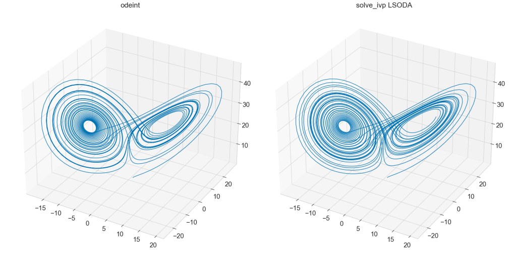 odeint and solve_ivp with identical integration method and temporal resolution. odeint and solve_ivp with identical integration method and temporal resolution.
Now both solutions have identical temporal resolution. But their solution is still not identical. I was unable to confirm why that is the case but I suspect very small floating point errors. The Lorenz attractor is a chaotic system and even small errors can make it diverge. The following plot shows the first variable of the system for odeint and solve_ivp from the above simulation. It confirms my suspicion that floating point accuracy is to blame but was unable to confirm the source. 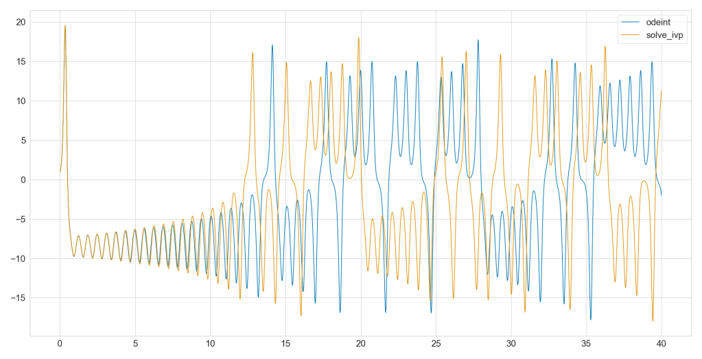 Solutions from odeint and solve_ivp diverge even for identical temporal resolution and integration method. Solutions from odeint and solve_ivp diverge even for identical temporal resolution and integration method.
There is one more way to make the system more smooth: decrease the tolerated error. We will not go into that here because it does not relate to the difference between odeint and solve_ivp. It can be used in both interfaces. There are some more subtle differences. For example, by default, odeint expects the first parameter of the problem to be the state and the second parameter to be time t. This is the other way around for solve_ivp. To make odeint accept a problem definition where time is the first parameter we set the parameter tfirst=True. In summary, solve_ivp offers several integration methods while odeint only uses LSODA. Share this:TwitterFacebookLike this:Like Loading... Related |
【本文地址】